
A case study in the limitations of deterministic withdrawal planning. A retiree whose return and inflation assumptions were realised almost exactly, yet whose corpus was exhausted seven years ahead of the projected horizon.
Deterministic Approach
Retirement planning is typically undertaken using the ‘deterministic’ approach. In this approach, retirement computations are undertaken using a single estimate for asset returns, inflation and retirement period. If you have previously used a typical retirement calculator, you would be familiar with these inputs.
The critical flaw in this approach is that it assumes that asset returns and inflation are predictable. This is why this approach is called 'deterministic', as it assumes that the future is determinable and predictable. Unless you have a crystal ball, this is not a good assumption.
The margin of error is significant in the deterministic approach because we are using point/single estimates for asset returns and inflation. If we are making one single prediction about the future, and that prediction turns out to be wrong, our retirement plan will be in trouble. Even if our prediction comes close to reality, small deviations will compound over a long retirement period (which can span multiple decades) and lead to a significant divergence.
As we will show in the case study that follows, even if we get our projections right, the deterministic approach is still problematic because it ignores volatility. Under deterministic computations, we assume that our retirement will face the same asset returns and inflation each year. Reality is of course very different. Each year will bring variation in equity returns, debt returns and inflation.
Stochastic Approach
A better method for retirement planning is to use the stochastic approach. A stochastic method will not provide a single outcome, but a range of possible outcomes. In this approach, your retirement portfolio is put through different scenarios of asset returns and inflation to check if it can last for the full retirement period (see Figure 1). Using the technique of simulation, we can run thousands of simulations on a retirement portfolio using varied equity returns, debt returns and inflation to check for the adequacy of a retirement corpus.
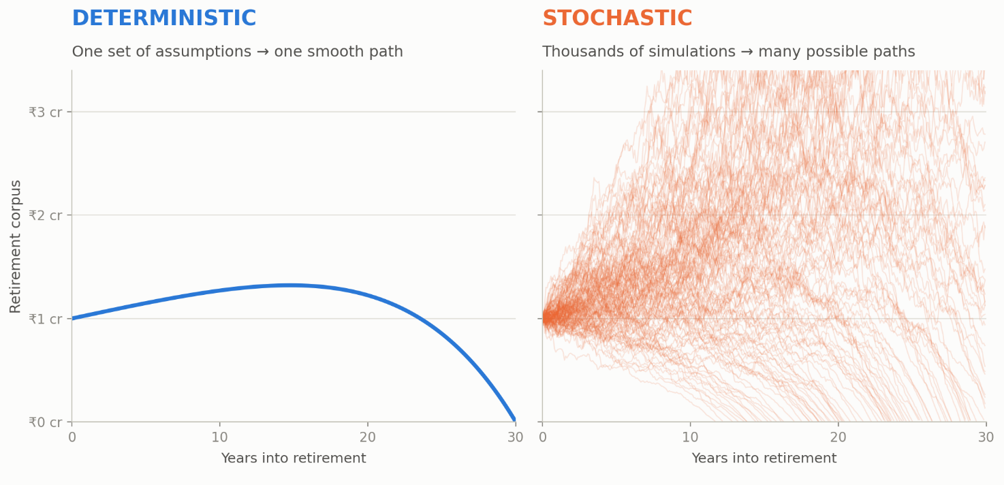
Figure 1 — Deterministic vs stochastic methods (illustrative)
Why this matters
To illustrate why this matters, let us take an example of our 1994 retiree. Arjun retires in the year 1994 with a retirement corpus of ₹ 1 crore and plans for a retirement with the below deterministic assumptions.
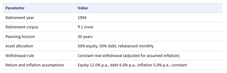
With the above parameters, he calculates the withdrawals using typical present value-future value formulas (in Excel, you can do this with the PMT formula) and arrives at a monthly withdrawal of approximately ₹46,0001 , which can be inflation adjusted every month. This corresponds to an annual withdrawal of about ₹ 5.52 lakhs and on a corpus of ₹ 1 crore, the withdrawal rate comes to 5.52%.
To test the robustness of this deterministic withdrawal rate, we can back-test Arjun’s retirement corpus from 1994 onwards using actual equity, debt and inflation2 data. Figure 2 shows the outcome of the back-test. The corpus exhausts in 2016, about 7 years before expectation.
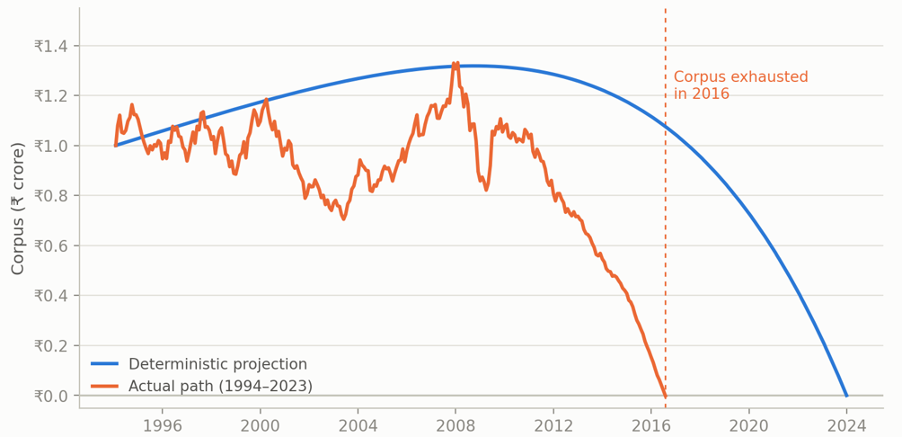
Figure 2 — Corpus path, deterministic vs stochastic
Initially, things worked out well. The stochastic (orange) line hovers around the deterministic (blue) line. But this proved to be the lull before the storm. During the dot-com bust in 2000, the markets tanked by more than 20%. The value of Arjun’s retirement portfolio deviated significantly from the projected value. Much to Arjun’s relief, the bull market during 2004-2007 took the retirement corpus close to the projected value by the end of 2007.
Then came the global financial crisis in 2008, which severely hit Arjun’s corpus (market fall of over 50%). Much to his dismay, the corpus did not recover from this shock. In every subsequent year, the gap between the projected and the actual corpus grew wider, and the corpus exhausted itself prematurely in 2016.
What went wrong?
Was Arjun’s return projections too aggressive? Not really. Realised portfolio return was higher than assumed. However, realised inflation was higher than projection as well. Netted, the realised real return on the portfolio was 3.73% p.a. against an assumed 3.77% p.a. Arjun got his return projections spot on (see Table 1). Yet he ran out of money prematurely.
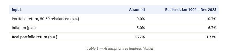
This outcome is because the deterministic method does not take into account volatility and path-dependence of returns and inflation. Retirement planners call this the sequence of return risk. It is important to consider not only the average return earned by a portfolio, but also the sequence in which those returns were earned. Two portfolios with the same average return can have wildly different terminal values depending on the sequence of returns earned (see Table 2).
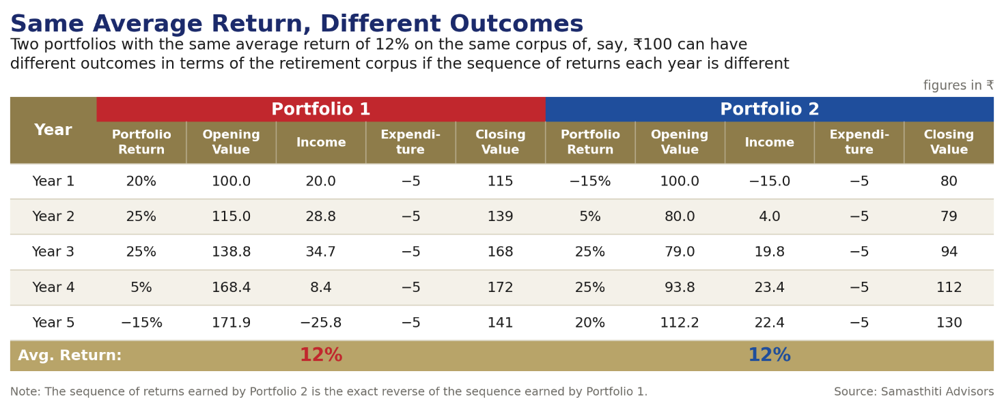
Table 2 — Sequence of Return Risk
What we need to remember
A deterministic answer sounds precise, but this precision is its biggest problem. The calculation hands you one path and makes no allowance for any deviation from that path. A stochastic approach gives you odds instead of a single number. Instead of one smooth path, it tests thousands of different ones and counts how often the money lasted. The useful answer is not “you can draw ₹46,000 a month.” It is “at this rate the money lasted in 95 runs out of 100, and here is what went wrong in the other five.”
Drawing out the distinction between deterministic and stochastic methods is not just an academic curiosity. One of these words is already governing your retirement plan. It is time to find out which one and make these terms a core part of your retirement planning. It’s high time.
Disclaimer: Nothing discussed in this article is investment advice of any sort. Always consult with your financial and other advisers before investing.
- Each annual assumption is converted to a compounded monthly equivalent — equity 12% to 0.95%, debt 6% to 0.49%, inflation 5% to 0.41% — giving a blended portfolio return of 0.72% a month at a 50:50 allocation, or 0.3091% a month after inflation. Applying the annuity (PMT) formula, for beginning of month, to a ₹1 crore corpus at 0.3091% over 360 months gives a first-year pension of about ₹46,000 a month (₹5.52 lakh a year), a starting withdrawal rate of roughly 5.5% on a corpus of ₹1 crore. ↩︎
- Equity return is proxied by Sensex, debt by 1-3 year average FD rates as published by RBI and inflation by CPI. ↩︎
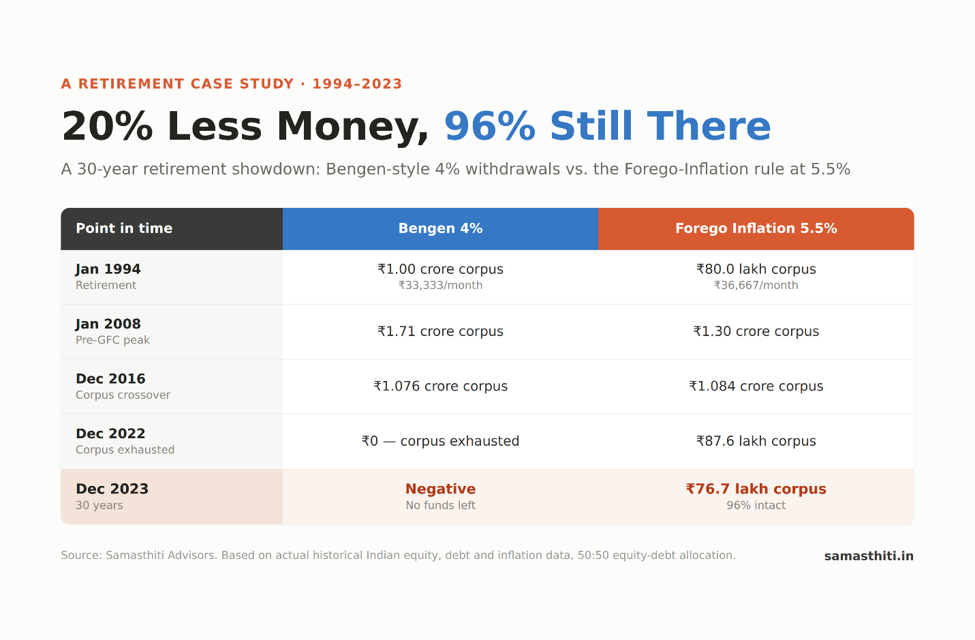
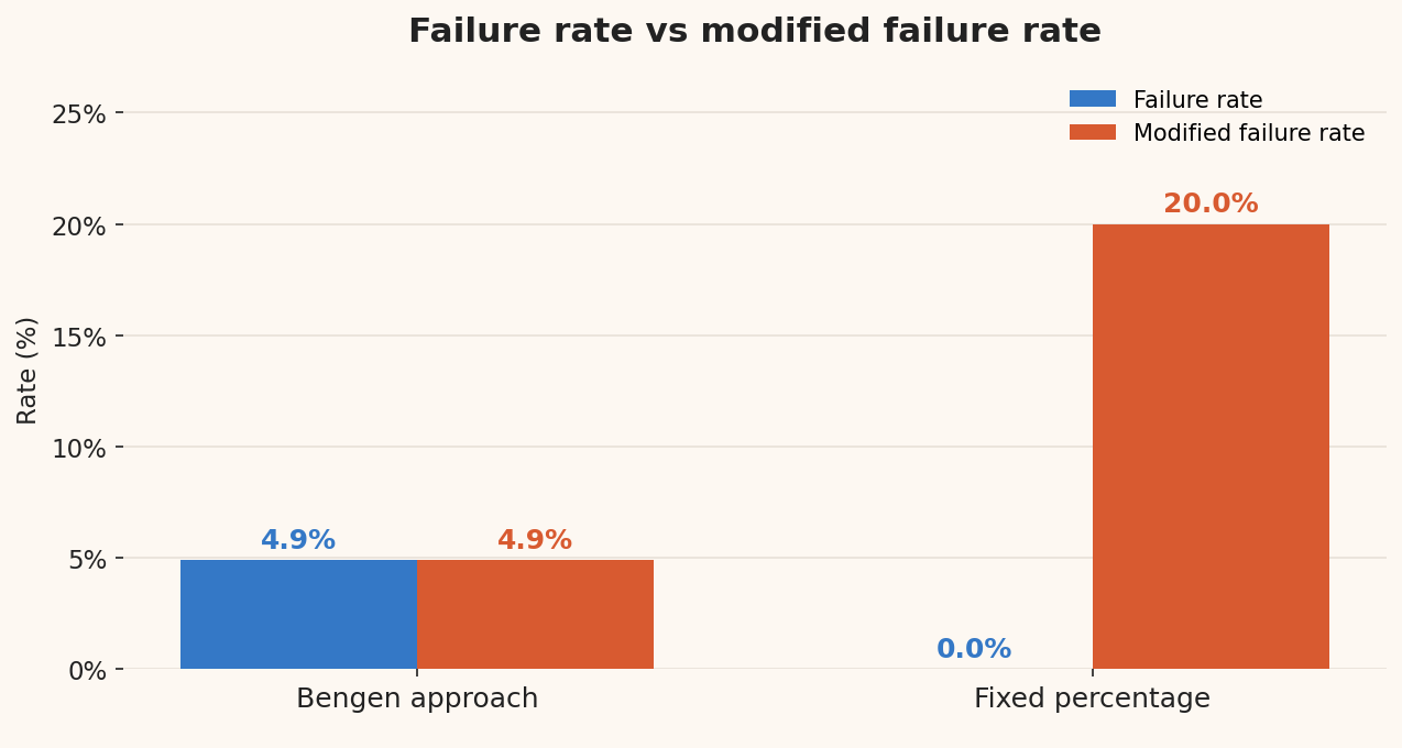
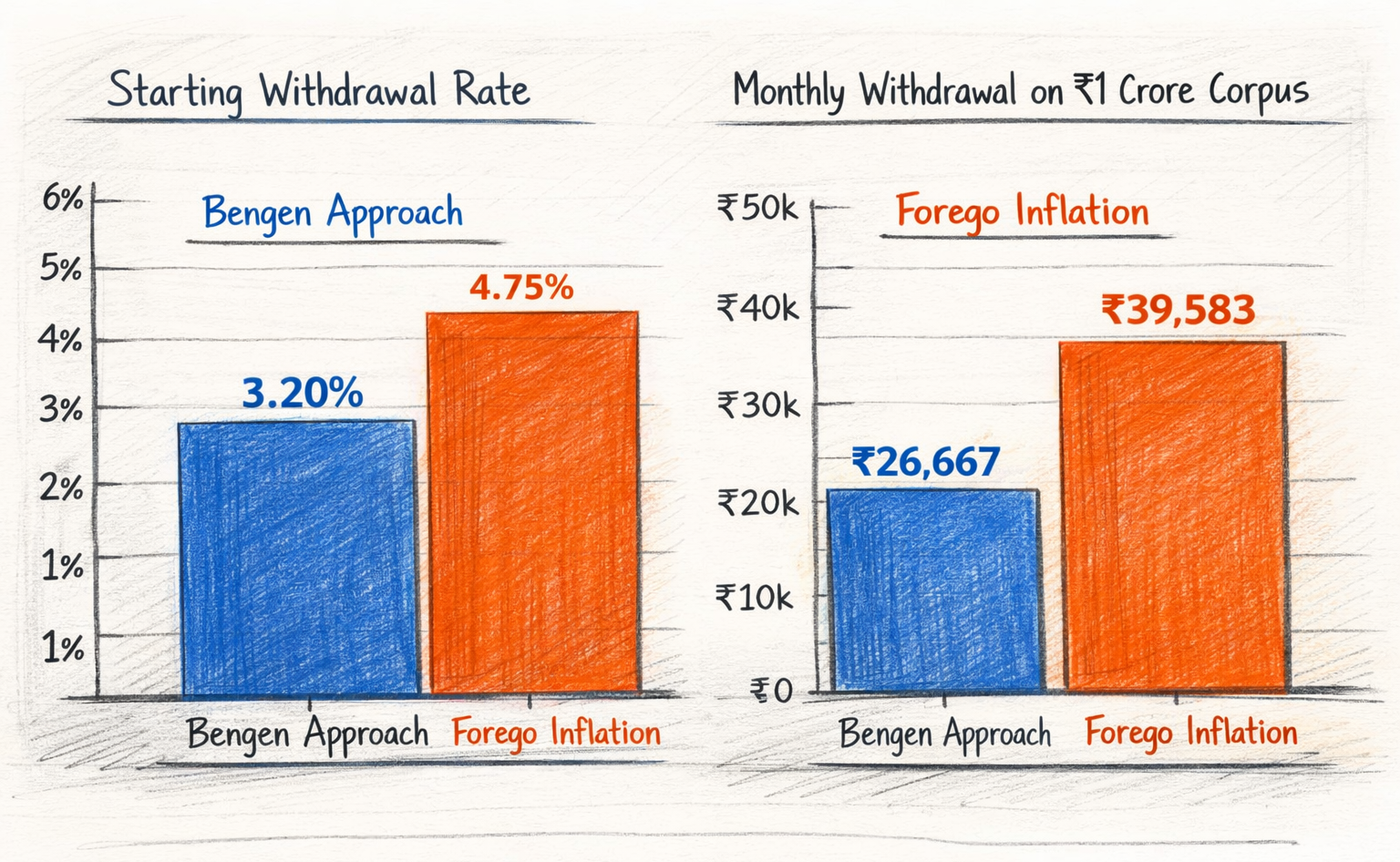


Grwat reasech. Thanks for this. Based on your analysis what is your conclusion based on your deep research about the safe withdrawl rate and what you suggest.
Thank you, you can look at a representative set of withdrawal rates here,
https://samasthiti.in/safe-withdrawal-rates-ready-reckoner/